Shapefiles to raster
Contents
Inside the Data-shp folder, you will find two sets of shapefiles. They are composed of several files and in order for them to work properly keep them all.
First, we will transform those shapefiles to Raster files with the help of rgdal.
#install.packages(c("rgdal","openxlsx") #only once
library(rgdal)
library(raster)
library(landscapemetrics)
library(tidyverse)
library(ggsci)
library(ggpubr)
library(openxlsx)
Read the shape files with readOGR.
try_map <- readOGR("Data-shp/GLYlanduse.shp") #read your filePlot the map.
plot(try_map)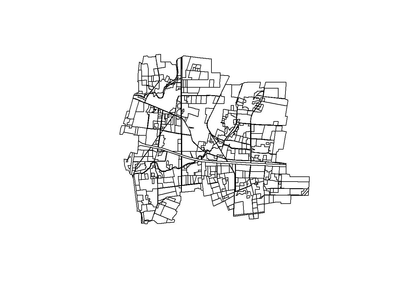
Currently, the map does not have a set of CRS so we will assign them to it because it is required for further analysis.This page has a lot of projections and CRS for your maps. R will require the text included in the Proj4 option, make sure you find your location or a CRS that includes the whole world like the following.
crs(try_map)
## CRS arguments: NA
newcrs <- CRS("+proj=merc +a=6378137 +b=6378137 +lat_ts=0.0 +lon_0=0.0 +x_0=0.0 +y_0=0 +k=1.0 +units=m +nadgrids=@null +wktext +no_defs")
crs(try_map)<-newcrs #add crs to a file
crs(try_map)
## CRS arguments:
## +proj=merc +a=6378137 +b=6378137 +lat_ts=0 +lon_0=0 +x_0=0 +y_0=0 +k=1
## +units=m +nadgrids=@null +wktext +no_defsCreate raster files
Set up a raster “template” to use in rasterize() so our shapefile can be transformed.
r <- raster(ncol=180, nrow=180)
extent(r) <- extent(try_map)
Rasterize the shapefile with rasterize make sure to have a target variable of a type double (numbers). The function str gives us the structure of any object. For specific parts of that object use $ and class
class(try_map$NUM)
## [1] "character"
We can see that NUM our variable for the raster is a character so we will need to change that before the raster of directly inside the function. We will do the last.
raster_map<-rasterize(try_map, r,as.double(try_map$NUM))# Transform NUM
class(raster_map)
## [1] "RasterLayer"
## attr(,"package")
## [1] "raster"
crs(raster_map)<-newcrs #add the crs
plot(raster_map)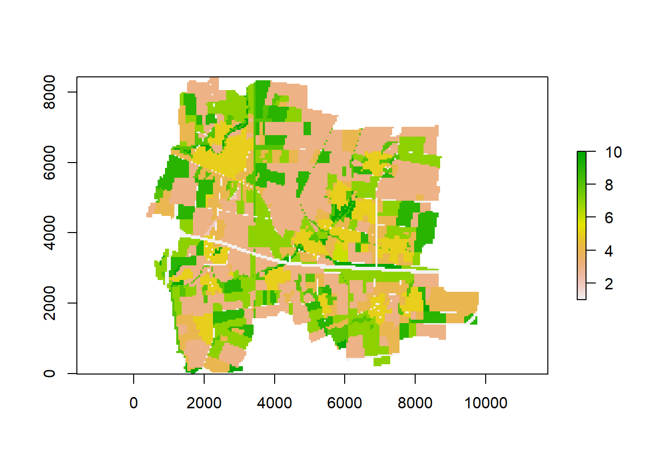
Export your new map with writeRaster
writeRaster(raster_map, "assigment.tif") #export the file- Try to do the same with the second map
GLYlanduseplan.shp
Activities
- Check your maps with
landscapemetrics::check_landscape() - Calculate one type of LSM for each level or 6, 4, and 2 LSM for the landscape, class, and patch level, respectively.
- Draw three graphs: one boxplot graph for all your class metrics, one bar graph for the landscape level, and one for the patch level metric with error bars showing standard error.
- Export your data files and figures.
Notes
- Try to use as fewer lines of code as possible. You can get all the landscape metrics results in 2 or 3 lines. If you want to have different data sets then 6 to 9 lines will be just right.
- Run both maps at the same time as instructed.
- To
rasterizethe other shapefile map you will need to use as.factor(map_landplan$TYPE)