Landscape Metrics
Contents
This page was created to provide an additional option to quantify landscape configuration using R. The landscape subject to analysis is powerful and can represent any spatial phenomenon. R will quantify, sample, show, and the areal extent and spatial configuration of patches within a landscape. We will cover a few important steps for data analysis and visualization. Firstly, an introduction to how to use the package, the functions it has, and how to extract the information. Secondly, we will take that information and create plots ready for publications so we can be more familiar with R and use some of the best features we can get from the program. All the code will be provided with a short explanation of what each line does.
Raster files are a great source of information, in our studies, they will determine the landuse type in each grid cell. Think of it as a large area made of a lot of squares, those squares will have a code (numbers) that tell the computer and us this has water, this has grassland, this has forests, etc.
GIS is one of the most used software for spatial analysis as it has a great interface for us to work with. Nevertheless, it is not the only one, R in the last few years is improving rapidly and is looking to implement better functions that can make analysis easier, wider, and above all reproducible. No matter your skills if you got R and the required packages you will be able to run what other people, improve and modify to your needs.
In order to use only R-studio for spatial analysis we will use, the package raster, it was created in R a long time ago and is one of the most solid packages for raster data analysis. We will learn a few functions that we will need when analyzing landscape metrics.
Let’s begin by loading our libraries, as mentioned before you will need to do this every time you restart your project or R.
library(raster)
library(sp)
library(landscapemetrics)
library(sf)
library(tidyverse)
library(ggsci)
library(ggpubr)
# If you get an error message saying: No such file or directory install the package first then run library
# If you are new to R then you can install the following packages
#install.packages(c("landscapemetrics","raster","sf","sp","tidyverse","rgdal", "scales","ggsci","plotrix","plyr"))
map<- raster("filename.tif") # your file name
plot(map) #to get a mapEverything you are going to do in R needs to be clear meaning that only what you tell the program to do will give you as output. We can begin by looking at our map, therefore, let’s use the builtin function for plotting plot.
library(raster)
beijing <- raster("data/map.tif")
plot(beijing)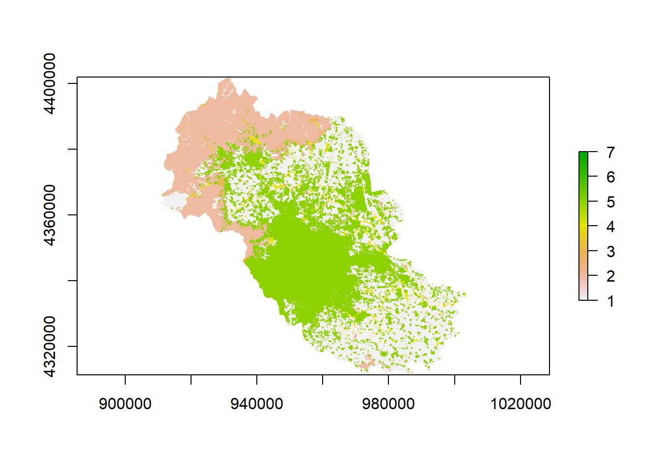
To determine the number of cells for each category we will use freq().
freq(beijing) # check the raster attributes
##      value  count
## [1,]     1 148909
## [2,]     2  90120
## [3,]     3   1733
## [4,]     4   9420
## [5,]     5 169928
## [6,]     7      9
## [7,]    NA 420626
Our raster map looks great and has the information that we want, therefore, we can take the metrics from this area.
Landscape Metrics
Landscapemetrics was introduced last year so we can say that it is a new package. It uses the same functions as other existing software to calculate landscape metrics but, it adds the R style that makes it better at integrating large workflows, tidy data format, small cell resolution, parametrization of metrics, and operable across operating platforms. In my personal opinion one package that will not give you headaches.
library(landscapemetrics)
check_landscape(beijing)
##   layer       crs units   class n_classes OK
## 1     1 projected     m integer         6  v
The function to get the metrics is calculate_lsm() and there are a few options for us to play with.
metrics_class_2020 <-calculate_lsm(beijing, #a raster object
                                   what=c("lsm_c_ai", # metric name
                                           "lsm_c_frac_mn", #  metric name
                                           "lsm_l_division",# metric name
                                           "lsm_l_pd")) # metric name
head(metrics_class_2020)
## # A tibble: 6 x 6
##   layer level class    id metric value
##   <int> <chr> <int> <int> <chr>  <dbl>
## 1     1 class     1    NA ai      89.4
## 2     1 class     2    NA ai      95.5
## 3     1 class     3    NA ai      78.9
## 4     1 class     4    NA ai      68.8
## 5     1 class     5    NA ai      91.3
## 6     1 class     7    NA ai      75
That is how it works. We got some metrics but what do they mean. You can open the full document of Landscapemetrics here and have a look at everything that the package can do.
First, remembering the names can be boring and complicated so we can take a look at the full list of metrics available in the package
metrics_names<-lsm_abbreviations_names #store the names
tail(metrics_names) #show the last 6 observations
## # A tibble: 6 x 5
##   metric name                      type                 level     function_name
##   <chr>  <chr>                     <chr>                <chr>     <chr>
## 1 sidi   simpson's diversity index diversity metric     landscape lsm_l_sidi
## 2 siei   simspon's evenness index  diversity metric     landscape lsm_l_siei
## 3 split  splitting index           aggregation metric   landscape lsm_l_split
## 4 ta     total area                area and edge metric landscape lsm_l_ta
## 5 tca    total core area           core area metric     landscape lsm_l_tca
## 6 te     total edge                area and edge metric landscape lsm_l_te
## levels(factor(metrics_names$type)) # Metrics types
view(metrics_names) # will open a new window with all the names
We can get all the metrics for the class, patch or landscape if we set a level. The metrics for all the levels if we only set a type like diversity metric,aggregation metric, shape metric, core area metric, area and edge metric, or complexity metric. If you leave them empty then you will get all the metrics for each map. The last may take a while it will depend on the capacity of your computer and how many maps you want to analyze.
class_metrics<-calculate_lsm(list(beijing), # add multiple maps
                             level = c("class"), #patch- landscape other options
                             type="aggregation metric") #get all the metrics for the given level
The workflow for this package is straightforward, we are able to get a lot of information for analysis and visualization
Utility functions
As mention by the authors, this part is one of the biggest differences over other software. We can visualize, extract, sample different areas for further analysis.
Visualization: Levels and Metrics
If we got all the information in one plot then it is hard to look at each class change and smaller changes are not obvious for the readers. The package includes a function that gives you the tools to select different level, class, and even metric. This is a great option to give a graphic meaning to our calculations. All will follow the structure show_
show_patches(beijing,labels = FALSE,class = 3) #shows the patches of class 3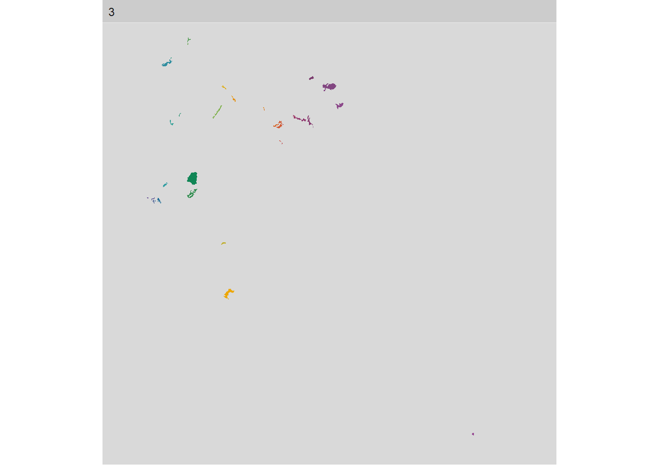
show_cores(beijing,labels = F,class = 2) #get the core areas of class 3 patches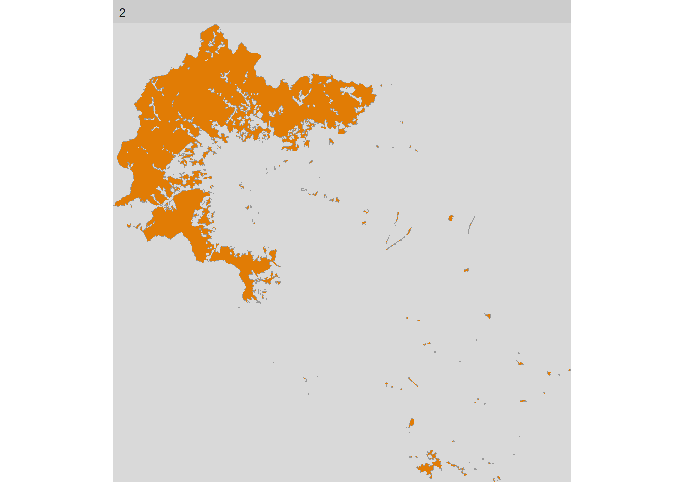
show_lsm(beijing,labels = F,class = 1,what = "lsm_p_area") #show the patches in colours based on the area, good to observe where that largest patch is located 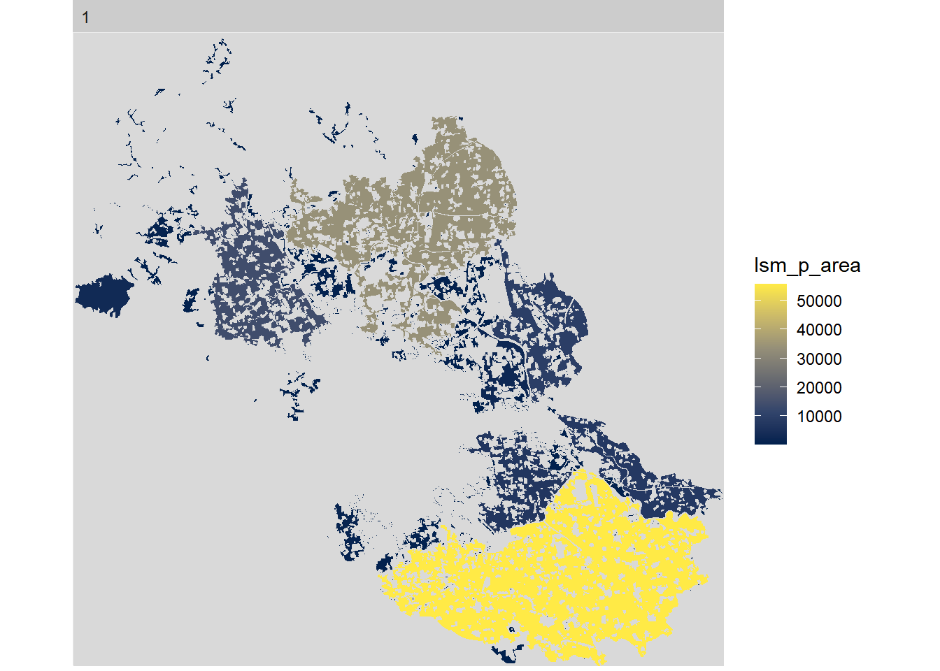
Buffer analysis
The first map was coded the right was for us, sometimes you may not get it that way and you will have results that are not right. let’s take a map with crs in latitude and longitude coordinates and get it ready for buffer analysis
sample_points <-matrix(c(932637.5, 4387377,
                        947509.5, 4368503),
                       ncol=2,byrow = TRUE)
sample_lsm(list(beijing), #map
                      what=c("lsm_c_pd"), #metrics
                      y = sample_points,  #points
                      size = 1500, #size
                      shape= "square") #shape of the buffer
## # A tibble: 7 x 8
##   layer level class    id metric value plot_id percentage_inside
##   <int> <chr> <int> <int> <chr>  <dbl>   <int>             <dbl>
## 1     1 class     1    NA pd     0.444       1               100
## 2     1 class     2    NA pd     0.111       1               100
## 3     1 class     4    NA pd     0.444       1               100
## 4     1 class     1    NA pd     0.556       2               100
## 5     1 class     2    NA pd     0.111       2               100
## 6     1 class     4    NA pd     0.222       2               100
## 7     1 class     5    NA pd     0.889       2               100
Moving window analysis
This will show a gradient of variability in the landscape. The analysis will go cell by cell, like a scanner, to determine how the center or focal cell changes in comparison to the neighboring cells. How different the surroundings are will give a higher value in that region and cell.
Large maps (many cells) will take a while to determine this function so we will just a small representation so you can get the results in a few seconds.
moving_window <- matrix(1, nrow = 5, ncol = 5) #set the extend of the analysis
moving_window
##      [,1] [,2] [,3] [,4] [,5]
## [1,]    1    1    1    1    1
## [2,]    1    1    1    1    1
## [3,]    1    1    1    1    1
## [4,]    1    1    1    1    1
## [5,]    1    1    1    1    1
result <- window_lsm(landscape, window = moving_window, what = c("lsm_l_pr", "lsm_l_np"))
Now lets plot the result and export the values if needed.
plot(result[[1]]$lsm_l_np) #plot(raster_file)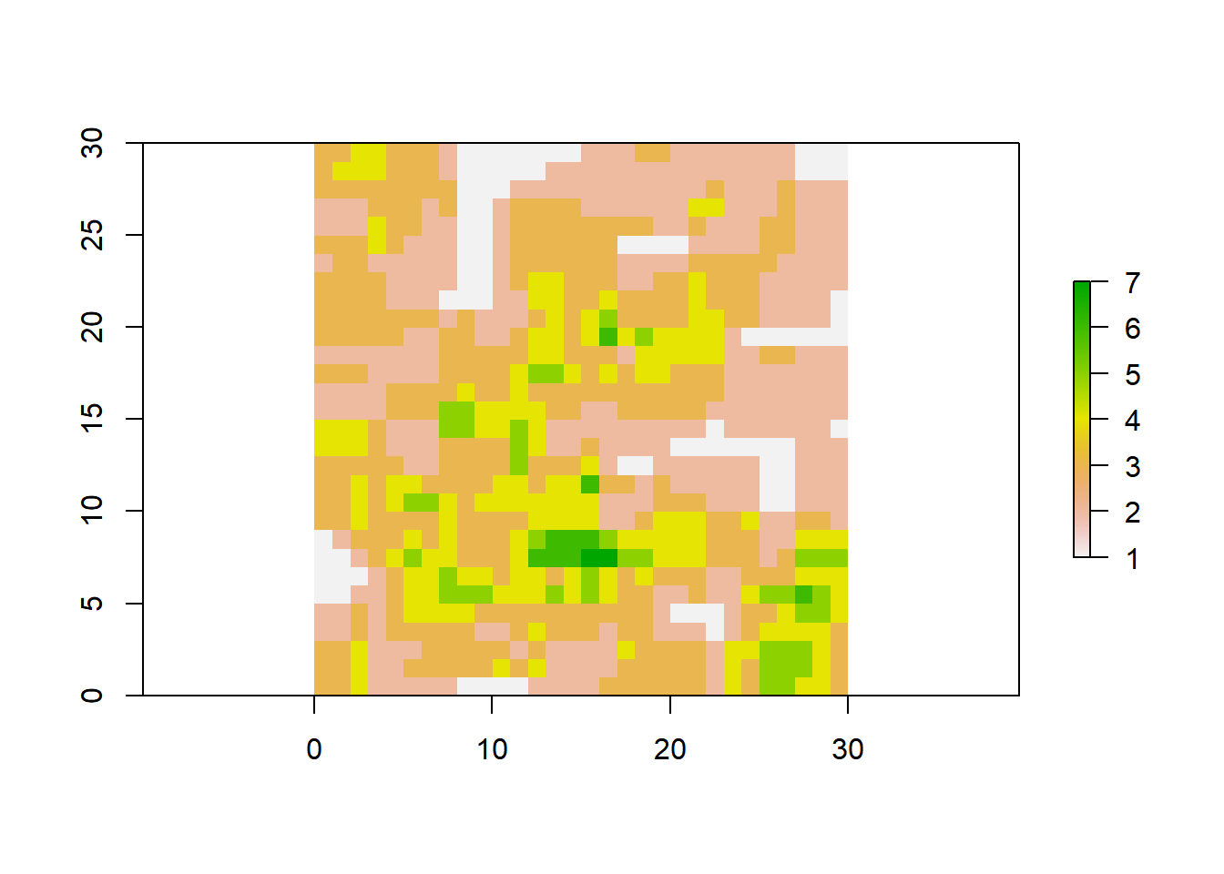
You can export the results after making a matrix matching the size of the raster file.
writeRaster(result[[1]]$lsm_l_np,"Moving window np.tiff",format="GTiff")These are the main functions of the package landscapemetrics, there are a lot more that you can explore in your own time. The results are clear and the structure is perfect for graphs, yet, we can make a few changes so they can be more informative to everyone and have great communication documents. Next, we will cover some other functions of R, data changes, graphs that we can carry out with these results.
Beyond the basic
Revalue and export
Let’s give the right names to our layers and classes.
metrics_class_2020$Year<- plyr::revalue(factor(metrics_class_2020$layer),c("1"="2000s")) # revalue and make a new variable
metrics_class_2020$land<-plyr::revalue(factor(metrics_class_2020$class),
                                       c("1"="Forest","2"="Built-up land",
                                         "3"="Cultivated Land","4"="Unused Land",
                                         "5"="Water Bodies","7"="Factories"))
data_frame $ variable means in the data_frame work in the x variable. Remember that we use
<-to store information so if we use the same name it will replace the old values. If we give a new name then we will have a new variable in that data set.Revalue your observations with the structure c(“old name”=“new name”) for as many different names you want to give.
We can reshape our data frame by metrics if you want to write tables with metrics as the columns and export that information.
metrics_class_2020s<-spread(metrics_class_2020[,c(5:8)],key =metric,value = value) #rows to columns by metric variable(key) and the values will take info from value variable
head(metrics_class_2020s,2) #show only the first 2 rows
## # A tibble: 2 x 6
##   Year  land             ai division frac_mn    pd
##   <fct> <fct>         <dbl>    <dbl>   <dbl> <dbl>
## 1 2000s Forest         89.4       NA    1.03    NA
## 2 2000s Built-up land  95.5       NA    1.05    NA
Export the data as a CSV file
write.csv(metrics_class_2020s,file = "metrics results.csv") #write a csv fileLatitude and longitude maps
As aforementioned, if our data is in degrees then we must transform the raster cells into meters. We covered buffer analysis, now, let’s deal with a more complex example doing multiple buffer sizes from a map and locations given to you in degrees.
First, both points and maps need to be in the same coordinates otherwise your sampling areas will not be accurate. For the sampling locations, we will cover two options, change the coordinates of the matrix, and then proceed to do the buffer analysis. Second, use the write function to set a gpkg file containing our points.
buffer_map<-raster("data/buffer/degree.tif")
#freq(buffer.map)
check_landscape(buffer_map) # look at the warning
## Warning: Caution: Coordinate reference system not metric - Units of results
## based on cellsizes and/or distances may be incorrect.
##   layer        crs   units   class n_classes OK
## 1     1 geographic degrees integer         6  x
The current map CRS
crs(buffer_map)
## CRS arguments: +proj=longlat +datum=WGS84 +no_defs
Get a CRS in m for your map and then use projectRaster function to project and save the map.
albers<-"+proj=aea +lat_0=0 +lon_0=105 +lat_1=25 +lat_2=47 +x_0=0 +y_0=0 +ellps=krass +units=m +no_defs" #a CRS for our map in meters
beijing_meters<-projectRaster(buffer_map,crs=albers,method ="ngb") # change the crs in a raster file make sure you add method='ngb'
check_landscape(beijing_meters) # now our map is ok
##   layer       crs units   class n_classes OK
## 1     1 projected     m integer         6  v
It is more likely to have sampling points in degrees therefore, we will need to give the CRS used to get those points then change that to the map CRS.
points<-read.csv("data/buffer/sample_points.csv") %>% #read a text file with longlat coordinates
  st_as_sf(coords = c("longitude", "latitude")) %>%  # make a spetial object of our points
  st_set_crs("+proj=longlat +datum=WGS84 +no_defs") # give them the coordinates
sample_points=st_transform(points,albers) #change the coordinates from degrees to m
sample_points
## Simple feature collection with 5 features and 2 fields
## geometry type:  POINT
## dimension:      XY
## bbox:           xmin: 932637.5 ymin: 4362892 xmax: 947509.5 ymax: 4387377
## CRS:            +proj=aea +lat_0=0 +lon_0=105 +lat_1=25 +lat_2=47 +x_0=0 +y_0=0 +ellps=krass +units=m +no_defs
##   X siteID                 geometry
## 1 1      1 POINT (932637.5 4387377)
## 2 2      2 POINT (935332.9 4369503)
## 3 3      3 POINT (935152.5 4362892)
## 4 4      4 POINT (947509.5 4368503)
## 5 5      5 POINT (947413.4 4368606)
A great option is to write a gpkg file for all your sample points.
st_write(points, "data/buffer/sample_points_m.gpkg") # saving the new object to a spatial data format GPKG
#read our points
sample_points = st_read("data/buffer/sample_points_m.gpkg", quiet = TRUE)
sample_points=st_transform(points,albers) #change the coordinates from degrees to m
sample_points
Great, both the map and the data are in the same units and projection so we can do the analysis for multiple buffer sizes.
buffer_sizes=c(500,750,1000,2000,3000) #we want buffers for this sizes

buffer_results = buffer_sizes %>% #buffer data
  set_names() %>% #use the given names
  map_dfr(~sample_lsm(list(beijing_meters), #map_dfr() return a data frame created by row-binding and column-binding respectively
                      what=c("lsm_c_pd","lsm_c_area_mn",
                             "lsm_l_shei","lsm_l_frac_mn"), #metrics
                      y = sample_points, #locations
                      size = .),  #from each element of the data
          .id = "buffer") #the variable name for each element of buffer_size

#write.csv(x = buffer_results,file = "Buffer analysis results.csv")
Use R graphics
R and the package ggplot2 are one of the best teams when we want to create incredible graphs. There are multiple reasons to use this package so this part will show you how to set the data and create great plots without the need to use other programs that can be simple but not reproducible.
levels(factor(buffer_results$buffer)) #look at the current order of the buffer data
## [1] "1000" "2000" "3000" "500"  "750"
buffer_results$buffer=factor(buffer_results$buffer,levels=c("500","750","1000","2000","3000")) #order the buffers
levels(factor(buffer_results$buffer))
## [1] "500"  "750"  "1000" "2000" "3000"
Change the classes and map.
buffer_results$class_name<-plyr::revalue(factor(buffer_results$class),c("1"="Grass","2"="Roads","3"="Rivers","4"="Forest","5"="City","6"="Open areas")) #name the classes
buffer_results$map<-plyr::revalue(factor(buffer_results$layer),c("1"="Beijing 2000")) #if multiple layers then change the name
Dplyr, similarly, to ggplot is part of the Tidyverse packages collection, and it is a package with a lot of functions created to restructure, modify, and arrange your datasets.
The functions have verbs that are easy to remember like filter summary group_by select we do not need to read the documents to know what they do. Let’s use those functions to get our plots. When using these functions you can also pipe both data and ggplot2 with %>% so you do not need to have one variable for the data set.
#get only the landscape observations
landscape_results<-filter(buffer_results,level=="landscape")
#plot a boxplot
ggplot(data=landscape_results,mapping=aes(x=buffer,y=value,fill=buffer))+
  geom_boxplot()+ #geometry you want to give to the data
  facet_grid(metric~.,scales = "free_y")+ #there are different plots
  scale_fill_aaas(alpha = 0.8)+ #fill colours
  theme_pubr() #plot theme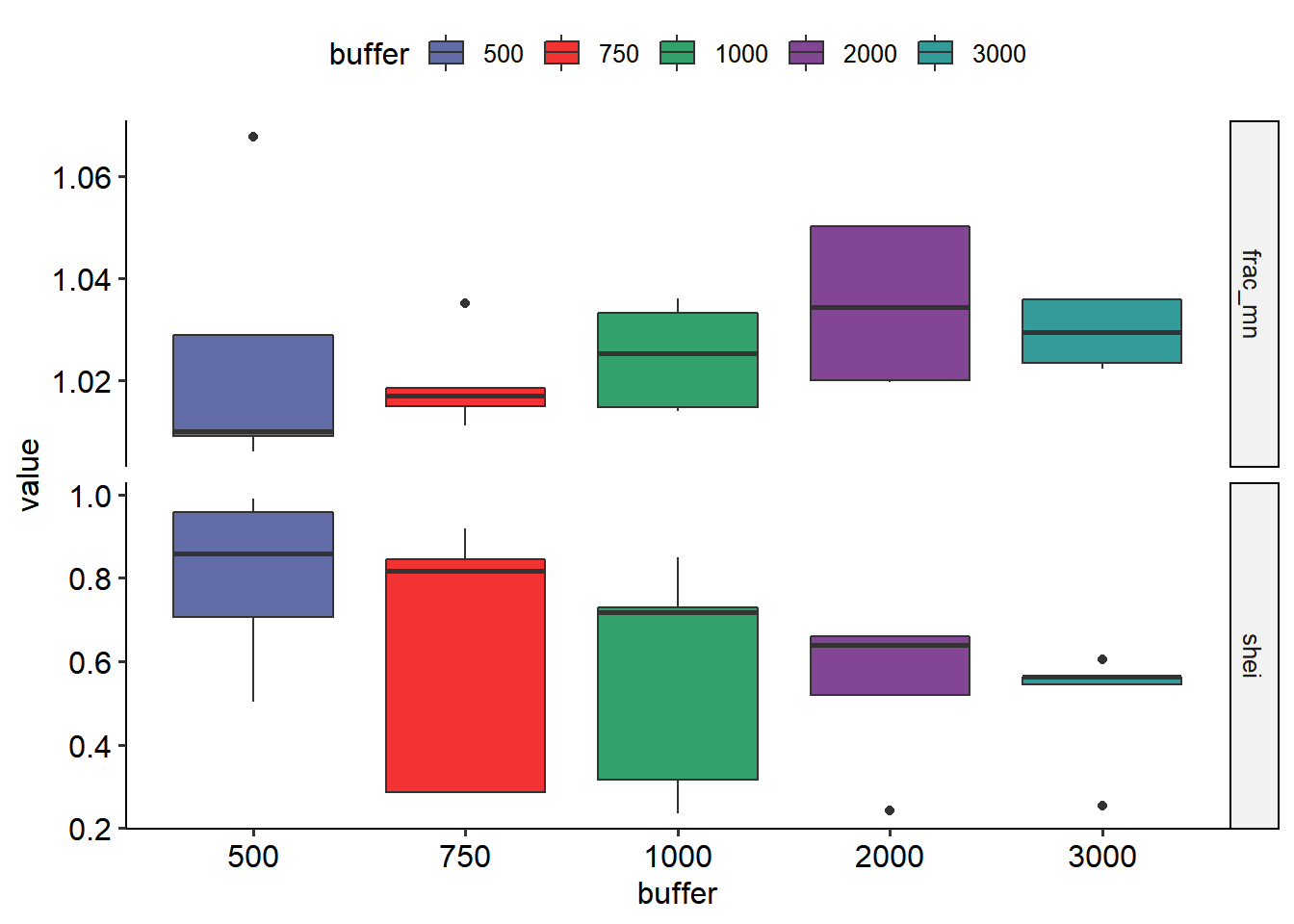
Now we will use more functions of dplyr for this plot.
p=filter(buffer_results,level=="class")%>%
  dplyr::select(c(1,4,6,7,9))%>% # select the variables that we need for the landscape group
  dplyr::group_by(buffer,class,metric)%>% # make a data set for each buffer and metric so it can give me a summary
  dplyr::summarise_all(funs(mean(.,na.rm=TRUE),  #mean of all the variables
                            sd(.,na.rm=TRUE), #sd of all the variables
                            se=plotrix::std.error(.,na.rm=TRUE)))%>% # standard error of all the variables
  ggplot(aes(x=class,y=value_mean,fill=factor(class)))+ #no need to add data=df because it is going to use the last step data
  geom_col()+
  geom_point(aes(fill=NULL,colour="Mean"),position = position_dodge2(width = 0.75,padding = 0),shape=15)+
  scale_colour_manual(values="black")+
  geom_errorbar(position = position_dodge2(width = 0.75,padding = 0.80),
                aes(y=value_mean,
                    ymax=value_mean+value_se,
                    ymin=value_mean-value_se))+
  facet_grid(metric~buffer,scales = "free",switch = "y", # flip the facet labels along the y axis from the right side to the left
             labeller = as_labeller( # redefine the text that shows up for the facets
               c(area_mn = "Mean Area",pd="PD(n/100/ha)",
                 "500"="500","750"="750","1000"="1000","2000"="2000","3000"="3000")))+
  scale_fill_jco(alpha = 0.7)+
  labs(x="Class",y=NULL,fill=element_blank(),colour=element_blank())+
  theme(panel.border = element_rect(linetype = "solid",fill=NA),
        panel.background = element_rect(fill = NA),
        panel.grid = element_line(colour="grey95",linetype = "dashed"),
        legend.background = element_blank(),
        axis.text=element_text(size=16, colour = "black"),
        legend.position ="bottom",
        legend.box = "horizontal",
        strip.background = element_blank(), # remove the background
        strip.placement = "outside",
        strip.text = element_text(size=13,colour="black"))
p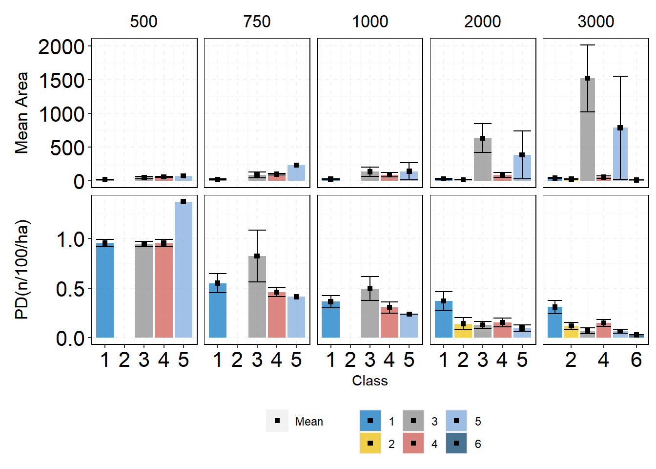
The plot is ready and we need to add some tags inside each facet and export it.
#this function will place letters inside each facet
tag_facet_inside=function(p, open = "", close = "", tag_pool = LETTERS, x = -Inf, y = Inf,
         hjust = -0.5, vjust = 1.5, fontface = 2, family = "", ...) {

  gb <- ggplot_build(p)
  lay <- gb$layout$layout
  tags <- cbind(lay, label = paste0(open, tag_pool[lay$PANEL], close), x = x, y = y)
  p + geom_text(data = tags, aes_string(x = "x", y = "y", label = "label"), ..., hjust = hjust,
                vjust = vjust, fontface = fontface, family = family, inherit.aes = FALSE)
}

tag_facet_inside(p, #ggplot2 object
                 x = 0.44, #place on the x axis
                 tag_pool = letters, #lowercase letters for the tags, LETTERS uppercase
                 size=4)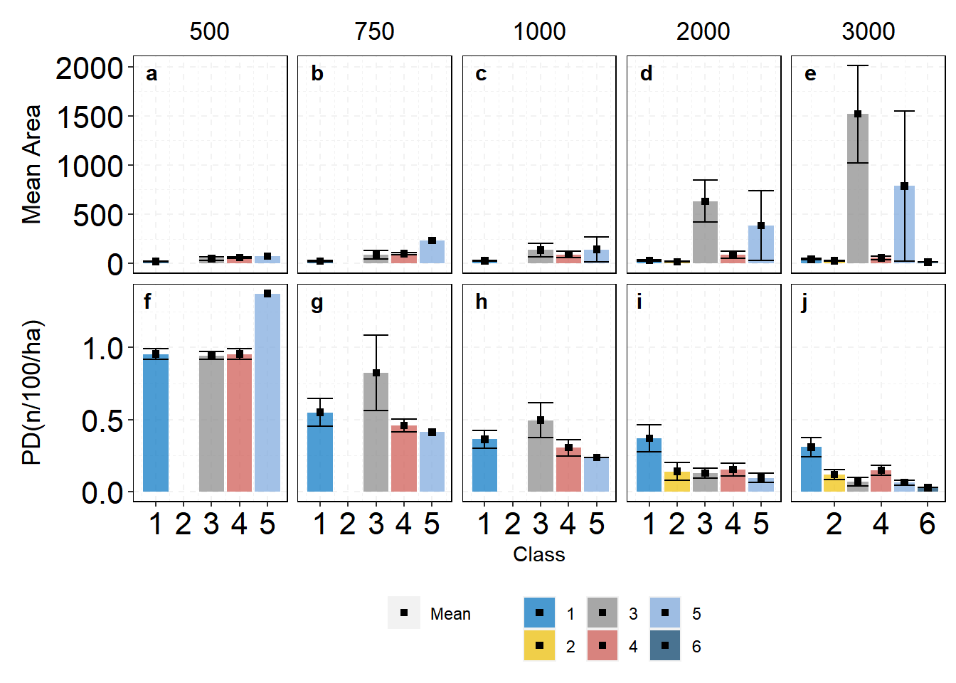
To export plots at a great resolution you will need the following lines of code.
ggsave(height = 8,width = 10, #dimensions
       filename = "buffer selected.png",
       dpi=600, #dots per inch, quality of the image (300-1000 journal requirements)
       device = "png") #device which will be used to save the plot
library(cowplot) # works better with word documents
cowplot::ggsave2(height = 8,width = 10,filename = "buffer selected.png",dpi=600,device = "png")